
A real SPICE engine in your browser.
Draw a schematic, press Run, read the result. Nothing to install, and nothing leaves your computer to be solved.
Analyses
Type the directive on the schematic, or pick it from the Run menu.
| Directive | What it does |
|---|---|
| .op | DC operating point: every node voltage and branch current at bias. |
| .dc | Sweeps a source and plots transfer curves and I-V characteristics. |
| .tran | Time domain with adaptive steps, starting from the operating point or from initial conditions. |
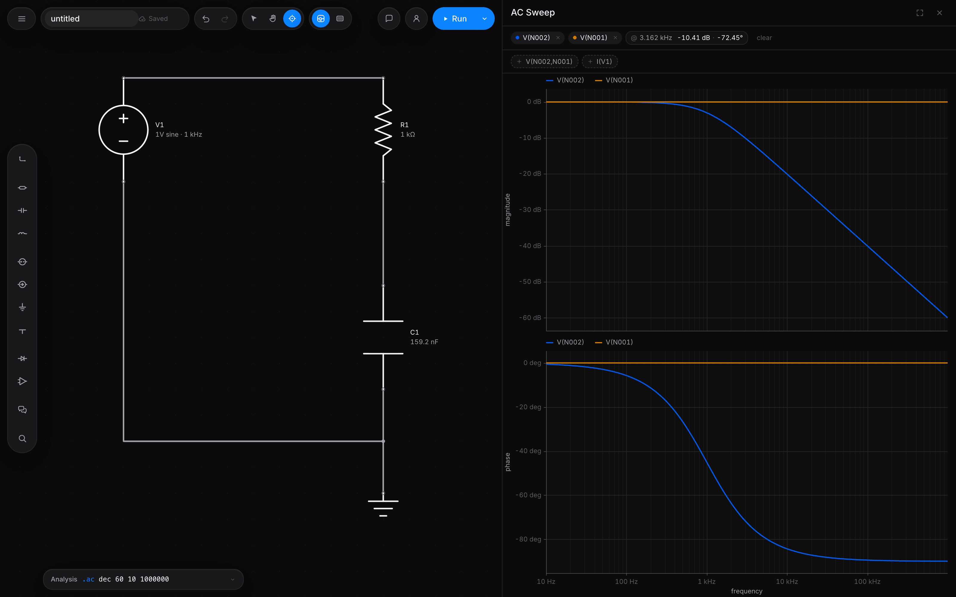
| .ac | Small-signal frequency response, linear, per decade or per octave, shown as a Bode plot. |
| .noise | Output and input-referred noise density across frequency. |
| .step | Repeats any analysis across component values, a .param or temperature, up to two nested axes. |
How it solves.
Modified nodal analysis with Newton-Raphson, junction limiting and gmin stepping, the method SPICE itself uses. The solver runs in a Web Worker, so the editor stays responsive during long runs.
A second opinion.
Any run can be repeated in ngspice, compiled to WebAssembly and running in the same tab. The two engines were written independently, so when they agree, the number means something.
Devices
- Passives
- Resistors with temperature coefficients, capacitors with ESR and initial conditions, inductors with series resistance, and coupled inductors.
- Sources
- DC and AC, with SIN, PULSE, PWL, EXP, SFFM and AM waveforms.
- Diodes
- Shockley junctions with junction limiting for robust convergence.
- BJTs
- Ebers-Moll with forward and reverse Early voltage.
- MOSFETs
- Level 1 with body effect, subthreshold conduction and overlap capacitances.
- Power MOSFETs
- The VDMOS model, with its intrinsic body diode and nonlinear gate-drain capacitance.
- JFETs
- Characterised from datasheet values, Idss and pinch-off.
- Switches
- Voltage and current controlled switches.
- Controlled sources
- Linear E, F, G and H sources, and behavioural B sources driven by expressions.
- Op-amps
- A macromodel with finite gain, gain-bandwidth, slew rate, input and output impedance, and rail limits.
- Transmission lines
- Ideal lossless lines with a characteristic impedance and delay.
- Subcircuits
- Reusable .subckt blocks, instantiated as many times as you need.
Reading the result
- Probes
- Click any node or part to plot its voltage or current. Suggested probes appear after each run.
- Cursors
- Two draggable cursors read values and differences straight off the curve.
- Bode and spectrum
- Magnitude and phase for AC runs, and an FFT view for transient ones.
- Export
- Waveforms as CSV or as an LTspice compatible .raw file.
Bring your files
- Import
- LTspice .asc, KiCad 6 and later, SPICE netlists, Falstad circuits, and .raw or CSV waveforms.
- Export
- SVG and PNG images, SPICE netlists, structural Verilog, and a bill of materials.
Checked in public.
4,169 checks pass across 9 suites, and 13 of 14 reference circuits agree with ngspice. The one that does not is listed, with the reason.
Known limits
- Transistor models
- MOSFETs are Level 1 and BJTs are Ebers-Moll. Right for coursework and board-level analog, not for on-chip design with foundry models.
- No harmonic balance
- Periodic steady state is reached by running .tran until the transient decays.
- No RF tooling
- No S-parameters or Smith charts. Transmission lines are ideal and lossless.
- THD floor
- Distortion below about 0.05% reflects the sampling of the transient record, not the circuit.